Influence of the background
The remaining gas in our simplified simulations id modeled as a
static background potential, which then is removed to mimic
gas-expulsion. We investigated if the shape of this potential has any
influence on the outcome of our results. We varied the potential from
an uniform sphere to a highly concentrated Plummer distribution but
our results showed that the answer of the star distribution (fractal
distribution with fractal dimension 1.6) is almost completely
independent to the shape of the gas potential. Simulations with the
same initial conditions of the stars formed similar denser
configurations before gas expulsion. This result was on one hand
reassuring that our simplified models are quite insensitive to the
choice of static potential and on the other hand allowed us to probe
different regions of the LSF, as concentrated backgrounds have more
remaining gas within the star distribution than e.g. an uniform
sphere.
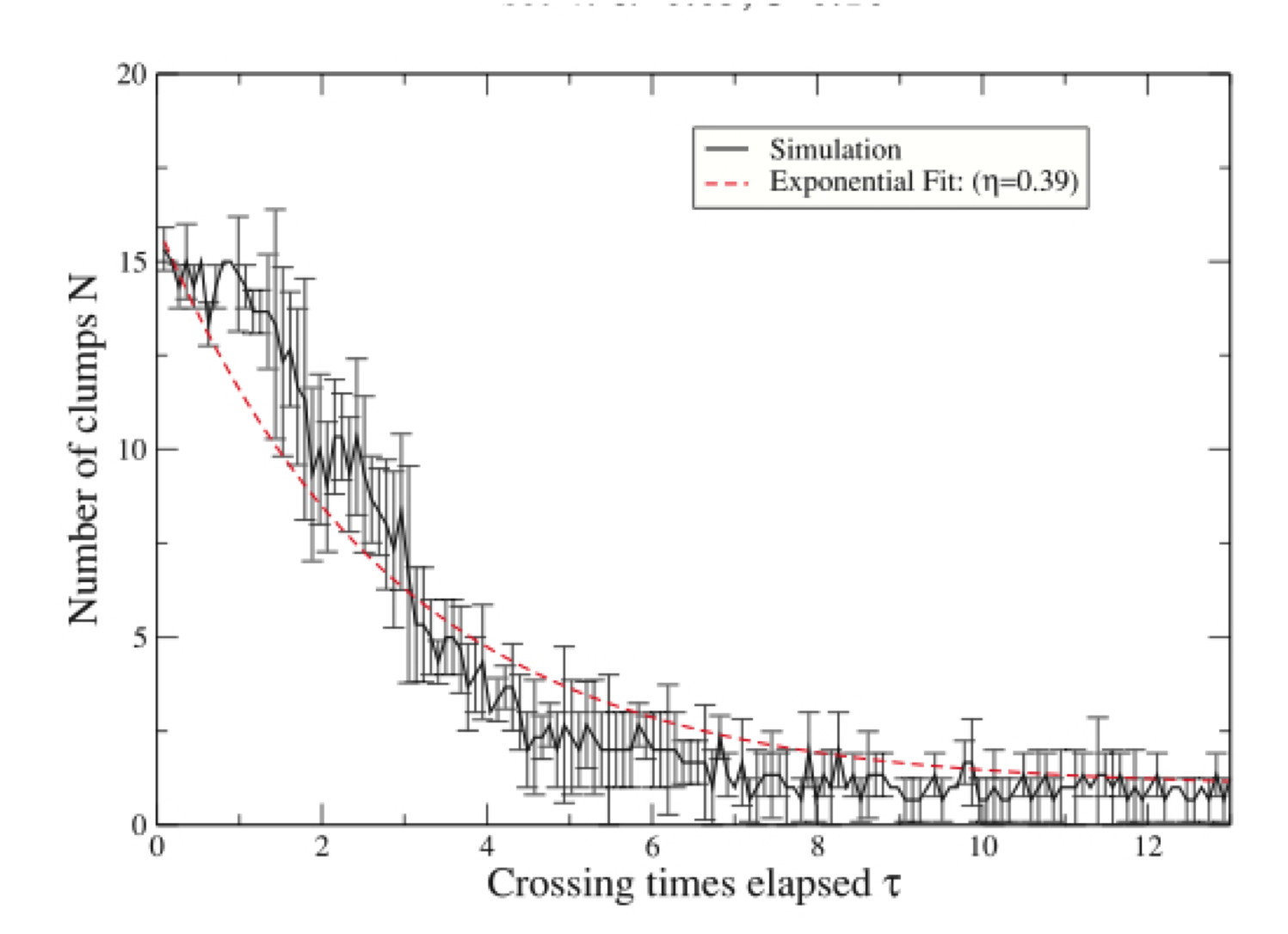
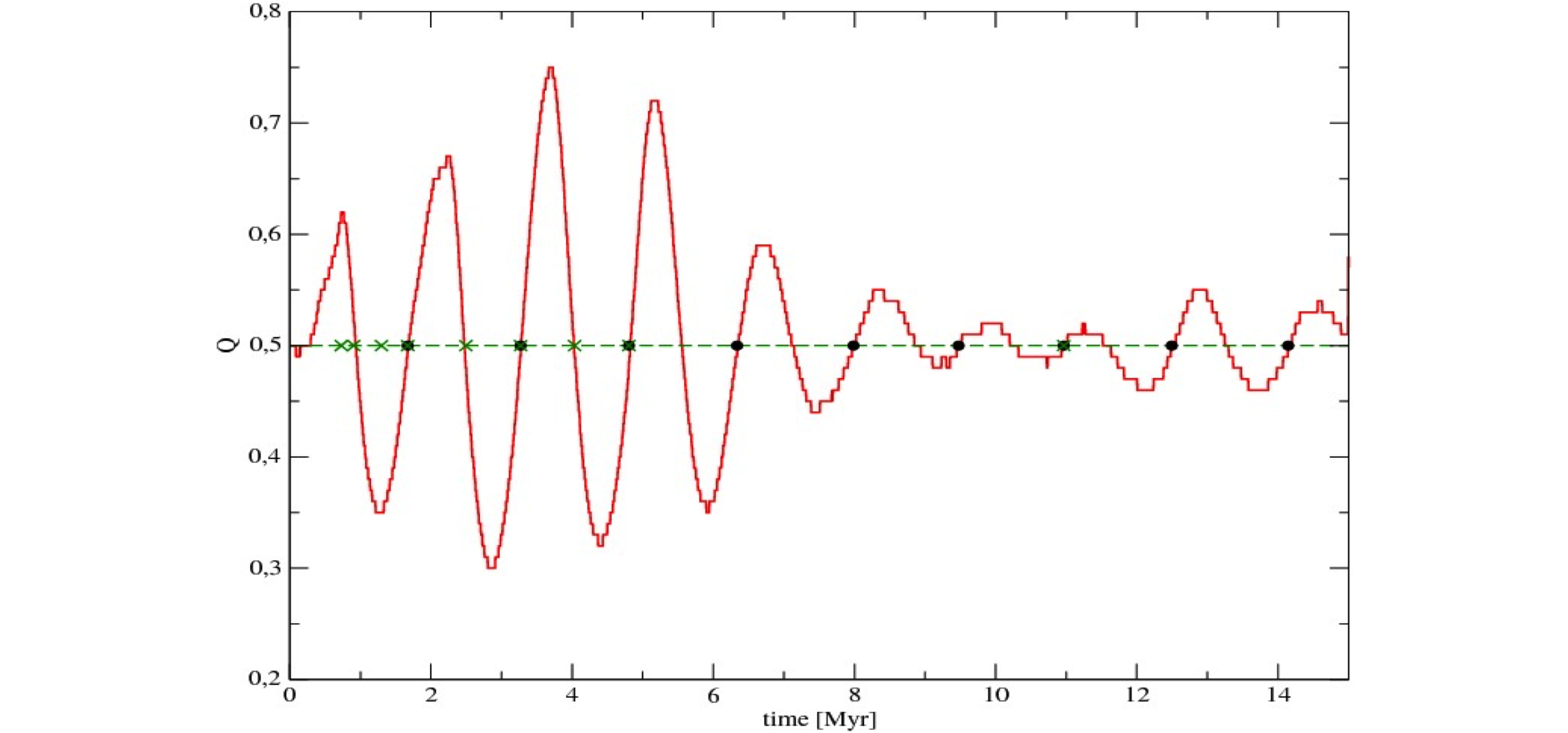
The Clumpiness parameter
The clumpiness parameter C describes how sub-structured a
distribution of stars is. As long as C < 0.8 we have a clumpy,
filamentary structure and C can be related with the fractal
dimension of the distribution and if C > 0.8 we have a smooth
distribution and C related directly to the shape (i.e.
concentration) of the distribution. We find that in our simulations
C changes from the fractal into the smooth regime at about the same
time we change from the 'chaotic' into the well behaved regime. This
happens at about 1.5 initial crossing times of the system or t_Q
approx 2 (see below).
The Snowball method
To analyse the data and determine the bound mass fraction we
developed a new tool, we call the 'Snowball method'. The method will
be described in detail in a paper, which we are preparing, to appear
in a refereed journal.
The influence of the IMF
Not truncated IMF
As stars do not have the same mass, we included now in our models a
standard Kroupa IMF (initial mass function) for stars between 0.1
and 120 M_sun. Even though there is observational and
theoretical evidence that the IMF in low-mass systems is truncated,
not just stochastically (i.e. a 50 M_sun star cluster cannot
harbour a 100 M_sun star and 30 M_sun star is highly
unlikely to be found in a 500 M_sun star cluster), but that
there is a certain maximum star mass for a given mass of the star
cluster, we first included only a stochastic truncation into our
models as we find it quite hard to determine which should be the mass
of our embedded cluster, as long as it is still in a fractal state.
We will postpone the investigation of truncated and varied IMFs to a
later stage of the project.
We see in our results, so far, that the internal evolution of the star
distribution is faster. Especially for dense systems, we find that
the bound fractions measured late are well below the trend we
determined for equal mass particles. A closer look to our results
then showed that this is due to the fast post-gas-expulsion evolution
of our low-N systems. Once we realised this fact, we started to
measure the bound fraction directly after the gas-expulsion and we
again recovered the trend shown in Eq.2.
Heavily mass-segregated models
As a first step into the investigation of mass-segregation we
performed models which are heavily mass-segregated, i.e. we place the
most massive star closest to the centre and the least massive one
furthest out. If this is a valid assumption, is debatable and we
will investigate also cases in which we have mass-segregated
sub-clumps (see reasoning for truncated IMF). What we see is that, as
predicted from stellar dynamics, the most massive stars form
immediately a tight binary in the central area. The results then are
a bit more counter-intuitive. Even though this hard binary ejects
many small stars from the system, a system with that binary survives
better than a system in which this binary gets ejected due to a
three-body encounter. In this sense we get different results than our
collaborators in the UK. We are still in the process to verify our
results.
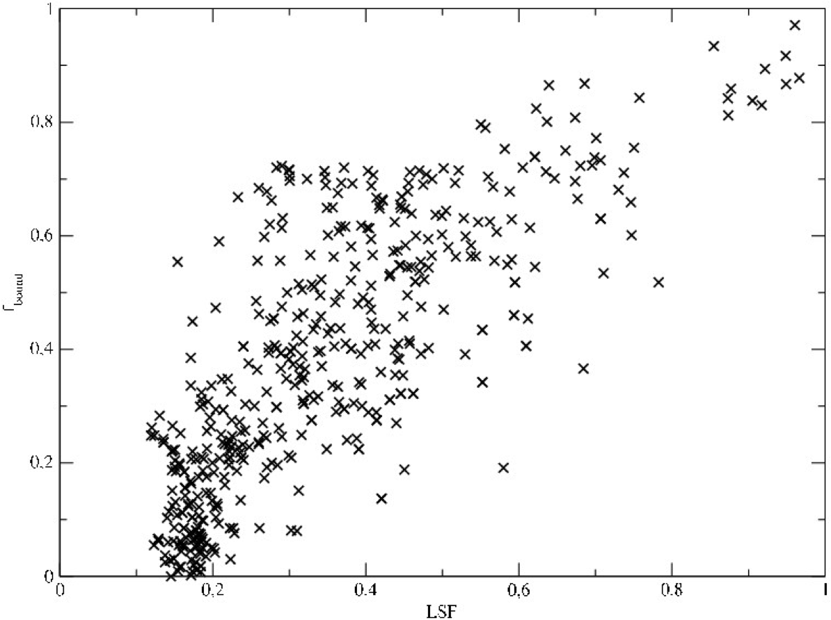
With many more simulations at hand, we see that the spread around our
theoretical curve is much larger than in the equal mass particle
simulations. If our theoretical model still holds will be subject to
investigations, which are in process.
Advanced SPH models
Latest Results
The direct N-body-SPH code Hybrid-Seren is still not ready to
produce results as the binary routines are not completely functional
yet. But the description paper is published with R. Smith as
co-author. In the meantime we make use of the AMUSE software
package which combines multiple purpose codes with a Phyton
envelope. With this we could combine a direct N-body code with an SPH
code to perform the first few test simulations (without feedback).
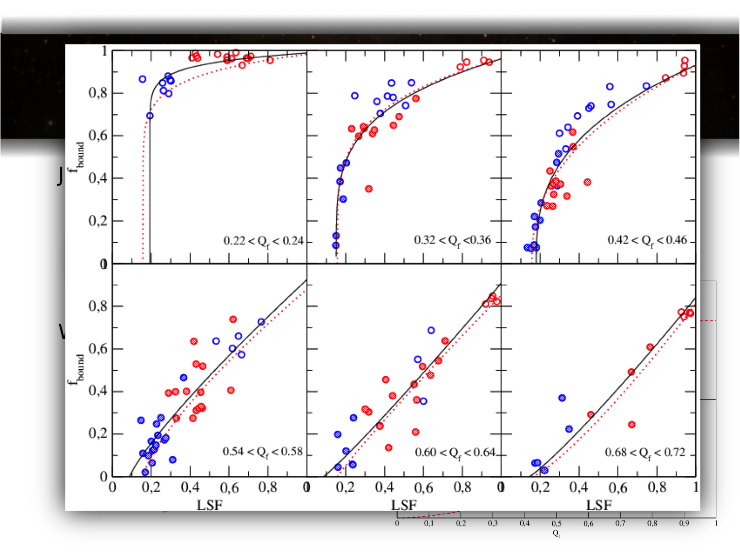
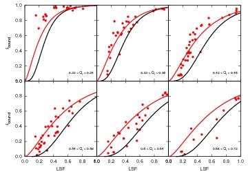
|
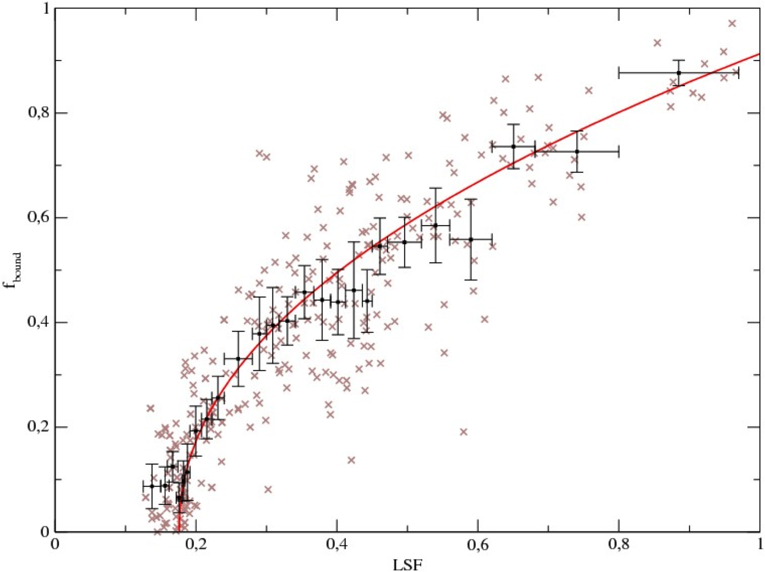
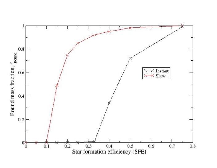 Fig.1: using data from
Baumgardt and Kroupa 2007
Fig.1: using data from
Baumgardt and Kroupa 2007
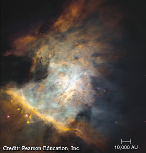
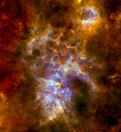
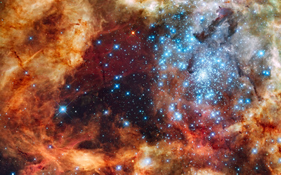
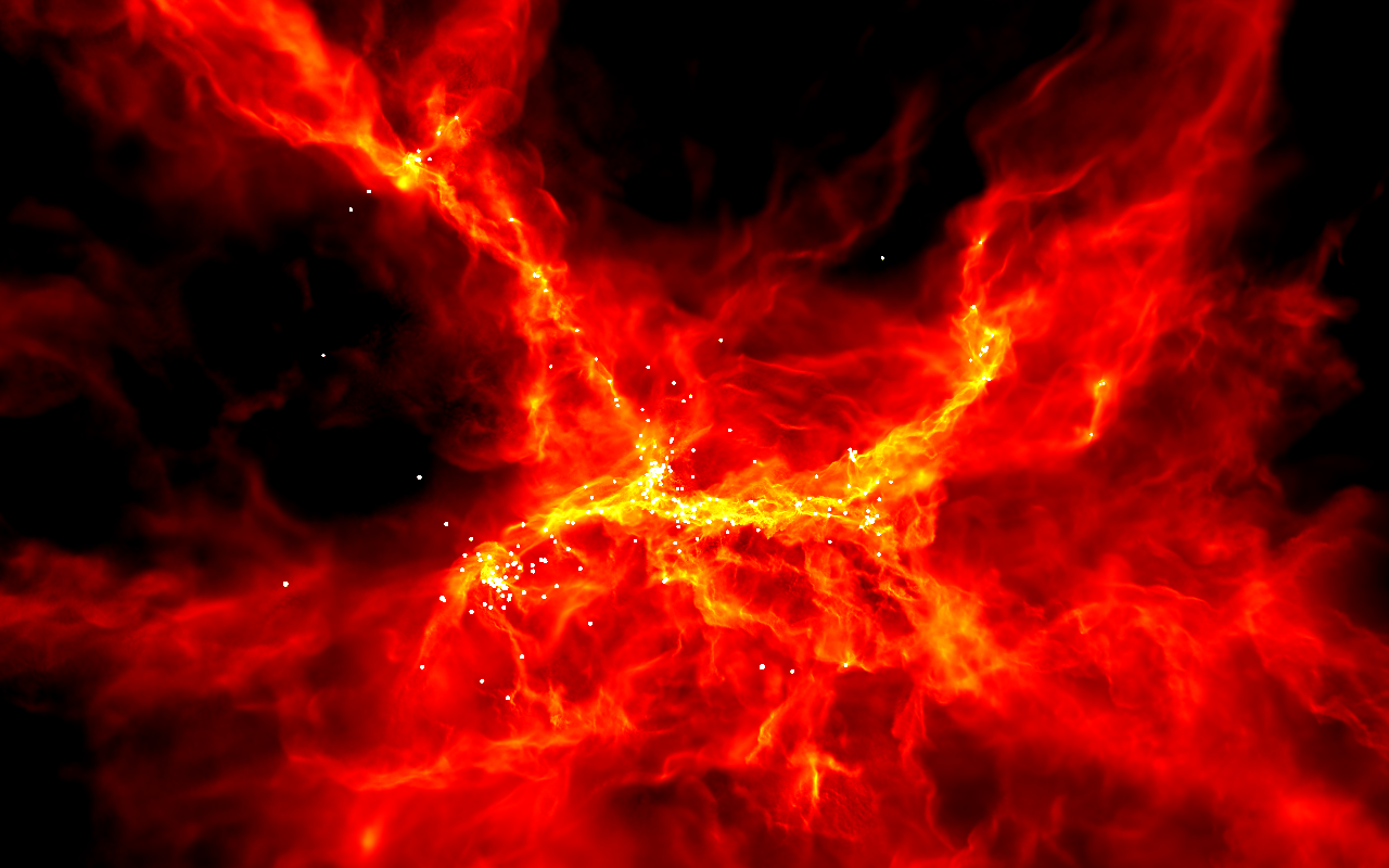
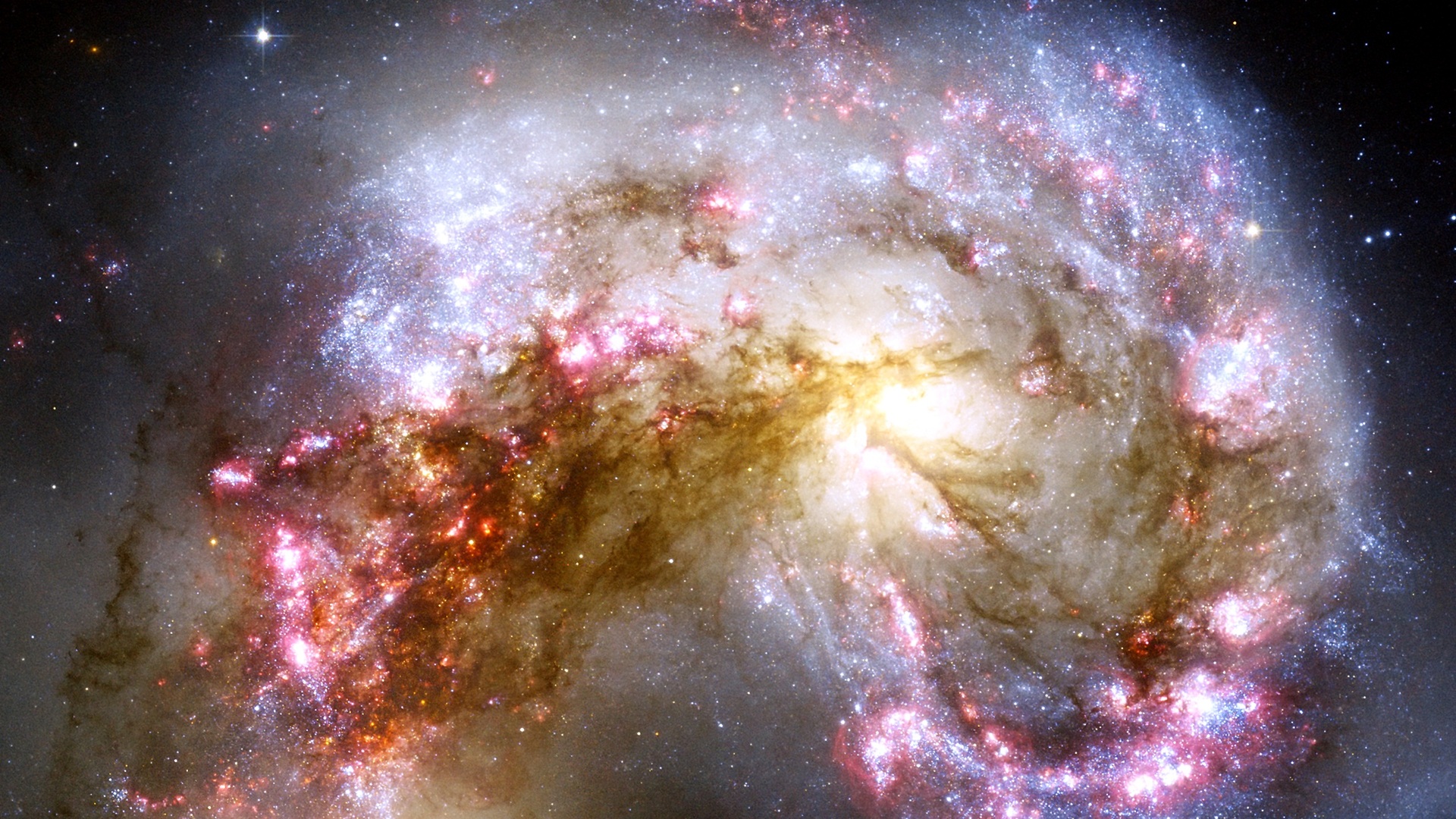 From top to bottom: The Orion nebular, the Carina star forming region, the
Tarantular nebular in the LMC and the cantral region of the Antennae
interacting galaxies.
From top to bottom: The Orion nebular, the Carina star forming region, the
Tarantular nebular in the LMC and the cantral region of the Antennae
interacting galaxies.
 credit: University of
Exeter
credit: University of
Exeter